Simulations

October 20 + 22, 2025

Author

Jo Hardin

Agenda 10/20/25

Why simulate?
Simulating to calculate probabilities
What makes a good simulation?

Data Conclusions

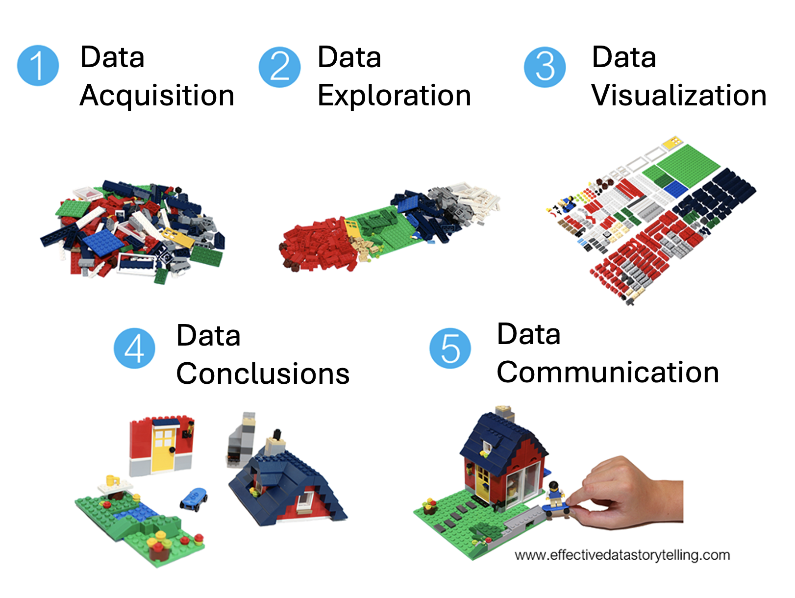
Based on https://www.effectivedatastorytelling.com/post/a-deeper-dive-into-lego-bricks-and-data-stories, original source: https://www.linkedin.com/learning/instructors/bill-shander

Simulate to…

… estimate probabilities (easier than calculus).
… understand complicated models.

Aside: `if_else()`

data.frame(value = c(-2:2)) |>
  mutate(abs_value = if_else(value >= 0, value, -value)) # abs val

  value abs_value
1    -2         2
2    -1         1
3     0         0
4     1         1
5     2         2

Aside: `case_when()`

set.seed(4747)
diamonds |>
  select(carat, cut, color, price) |>
  sample_n(20) |>
  mutate(
    price_cat = case_when(
      price > 10000 ~ "expensive",
      price > 1500 ~ "medium",
      TRUE ~ "inexpensive"
    )
  )

# A tibble: 20 × 5
   carat cut       color price price_cat  
   <dbl> <ord>     <ord> <int> <chr>      
 1  1.23 Very Good F     10276 expensive  
 2  0.35 Premium   H       706 inexpensive
 3  0.7  Good      E      2782 medium     
 4  0.4  Ideal     D      1637 medium     
 5  0.53 Ideal     G      1255 inexpensive
 6  2.22 Ideal     G     14637 expensive  
 7  0.3  Ideal     G       878 inexpensive
 8  1.05 Ideal     H      4223 medium     
 9  0.53 Premium   E      1654 medium     
10  1.7  Ideal     H      7068 medium     
11  0.31 Good      E       698 inexpensive
12  0.31 Ideal     F       840 inexpensive
13  1.03 Ideal     H      4900 medium     
14  0.31 Premium   G       698 inexpensive
15  1.56 Premium   G      8858 medium     
16  1.71 Premium   G     11032 expensive  
17  1    Good      E      5345 medium     
18  1.86 Ideal     J     10312 expensive  
19  1.08 Very Good E      3726 medium     
20  0.31 Premium   E       698 inexpensive

Aside: `sample()`

sampling, shuffling, and resampling: sample()

set.seed(47)
alph <- letters[1:10]
alph

 [1] "a" "b" "c" "d" "e" "f" "g" "h" "i" "j"

sample(alph, size = 5, replace = FALSE) # sample (e.g., from a population)

[1] "i" "b" "g" "d" "a"

sample(alph, size = 5, replace = TRUE) # sample (e.g., from a population)

[1] "j" "g" "f" "i" "f"

sample(alph, size = 10, replace = FALSE) # shuffle

 [1] "f" "h" "i" "e" "g" "d" "c" "j" "b" "a"

sample(alph, size = 10, replace = TRUE) # resample

 [1] "e" "j" "e" "b" "e" "c" "f" "a" "e" "a"

Aside: `set.seed()`

What if we want to be able to generate the same random numbers (here on the interval from 0 to 1) over and over?

set.seed(4747)
runif(4, 0, 1) # random uniform numbers

[1] 0.1949071 0.3390270 0.5147919 0.4516470

set.seed(123)
runif(4, 0, 1) # random uniform numbers

[1] 0.2875775 0.7883051 0.4089769 0.8830174

set.seed(4747)
runif(4, 0, 1) # random uniform numbers

[1] 0.1949071 0.3390270 0.5147919 0.4516470

Example 1: Alex & Jordan

Consider a situation where Alex and Jordan plan to meet to study in their college campus center (Mosteller 1987; Baumer et al. 2021). They are both impatient people who will wait only 10 minutes for the other before leaving.

But their planning was incomplete. Alex said, “Meet me between 7 and 8 tonight at the student center.” When should Jordan plan to arrive at the campus center? And what is the probability that they actually meet?

Simulate their meeting

Assume that Alex and Jordan are both equally likely to arrive at the campus center anywhere between 7pm and 8pm.

meet_func <- function(nada) {
  data.frame(
    alex = runif(1, min = 0, max = 60),
    jordan = runif(1, min = 0, max = 60)
  ) |>
    mutate(
      result = if_else(abs(alex - jordan) <= 10, "They meet", "They do not")
    )
}

n <- 100000

tic()
meet_map <- 1:n |>
  map(meet_func) |>
  list_rbind()
toc()

34.212 sec elapsed

tic()
meet_for <- data.frame()
for (i in c(1:n)) {
  meet_for <- meet_for |>
    rbind(
      data.frame(
        alex = runif(1, min = 0, max = 60),
        jordan = runif(1, min = 0, max = 60)
      ) |>
        mutate(
          result = if_else(abs(alex - jordan) <= 10, "They meet", "They do not")
        )
    )
}
toc()

149.679 sec elapsed

tic()
meet_vect <- data.frame(
  alex = runif(n, min = 0, max = 60),
  jordan = runif(n, min = 0, max = 60)
) |>
  mutate(result = if_else(abs(alex - jordan) <= 10, "They meet", "They do not"))
toc()

0.002 sec elapsed

Results

The results themselves are equivalent. Differing values due to randomness in the simulation.

meet_map |>
  group_by(result) |>
  summarize(number = n()) |>
  mutate(proprotion = number / sum(number))

# A tibble: 2 × 3
  result      number proprotion
  <chr>        <int>      <dbl>
1 They do not  69600      0.696
2 They meet    30400      0.304

meet_for |>
  group_by(result) |>
  summarize(number = n()) |>
  mutate(proprotion = number / sum(number))

# A tibble: 2 × 3
  result      number proprotion
  <chr>        <int>      <dbl>
1 They do not  69408      0.694
2 They meet    30592      0.306

meet_vect |>
  group_by(result) |>
  summarize(number = n()) |>
  mutate(proprotion = number / sum(number))

# A tibble: 2 × 3
  result      number proprotion
  <chr>        <int>      <dbl>
1 They do not  69529      0.695
2 They meet    30471      0.305

Visualizing the meet up

meet_map |>
  ggplot(aes(x = jordan, y = alex, color = result)) +
  geom_point(alpha = 0.3) +
  geom_abline(intercept = 10, slope = 1) +
  geom_abline(intercept = -10, slope = 1) +
  scale_color_brewer(palette = "Paired")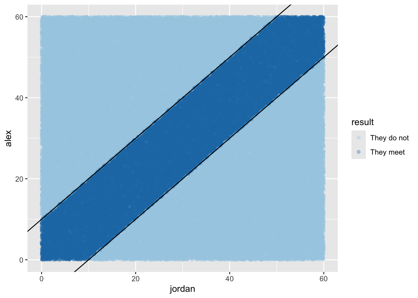

Example 2: hats

10 people are at a party, and all of them are wearing hats. They each place their hat in a pile; when they leave, they choose a hat at random. What is the probability at least one person selected the correct hat?

Step 1: representing the hats

hats <- c(1:10)
hats

 [1]  1  2  3  4  5  6  7  8  9 10

Step 2: everyone draws a hat

set.seed(47)
random_hats <- sample(hats, size = 10, replace = FALSE)

hats

 [1]  1  2  3  4  5  6  7  8  9 10

random_hats

 [1]  9  2  7  4  1 10  6  3  5  8

Step 3: who got their original hat?

hats == random_hats

 [1] FALSE  TRUE FALSE  TRUE FALSE FALSE FALSE FALSE FALSE FALSE

# TRUE is 1, FALSE is 0
sum(hats == random_hats)

[1] 2

# did at least one person get their hat?
sum(hats == random_hats) > 0

[1] TRUE

Code so far

set.seed(47)
hats <- c(1:10)
random_hats <- sample(hats, size = 10, replace = FALSE)
sum(hats == random_hats) > 0

[1] TRUE

Do we have a good estimate of the probability of interest?

Function

remove the magic number 10

hat_match <- function(n) {
  hats <- c(1:n)
  random_hats <- sample(hats, size = n, replace = FALSE)
  sum(hats == random_hats) > 0
}

hat_match(10)

[1] TRUE

hat_match(47)

[1] TRUE

Iterate

map_lgl(c(1:10), \(z) hat_match(n = 10))

 [1]  TRUE FALSE FALSE  TRUE  TRUE  TRUE  TRUE  TRUE FALSE  TRUE

map_lgl(c(1:10), \(z) hat_match(n = 10)) |>
  mean()

[1] 0.5

Reproducible

set.seed(4747)
num_iter <- 10000

map_lgl(c(1:num_iter), \(z) hat_match(n = 10)) |>
  mean()

[1] 0.6329

set.seed(123)
num_iter <- 10000

map_lgl(c(1:num_iter), \(z) hat_match(n = 10)) |>
  mean()

[1] 0.6333

Vary number of hats

hat_match_prob <- function(n, reps) {
  prob <- map_lgl(c(1:reps), \(z) hat_match(n = n)) |>
    mean()
  return(data.frame(match_prob = prob, num_hats = n))
}

hat_match_prob(47, 200)

  match_prob num_hats
1       0.62       47

Vary number of hats

hat_match_prob <- function(n, reps) {
  prob <- map_lgl(c(1:reps), \(z) hat_match(n = n)) |>
    mean()
  return(data.frame(match_prob = prob, num_hats = n))
}

set.seed(47)
map(c(1:20), hat_match_prob, reps = num_iter) |>
  list_rbind()

   match_prob num_hats
1      1.0000        1
2      0.4964        2
3      0.6695        3
4      0.6241        4
5      0.6376        5
6      0.6290        6
7      0.6299        7
8      0.6299        8
9      0.6373        9
10     0.6273       10
11     0.6319       11
12     0.6348       12
13     0.6393       13
14     0.6300       14
15     0.6280       15
16     0.6396       16
17     0.6355       17
18     0.6283       18
19     0.6304       19
20     0.6461       20

Visualizing

set.seed(47)
num_iter <- 10000
map(c(1:20), hat_match_prob, reps = num_iter) |>
  list_rbind() |>
  ggplot(aes(x = num_hats, y = match_prob)) +
  geom_line() +
  labs(y = "probability of at least one match", x = "number of hats")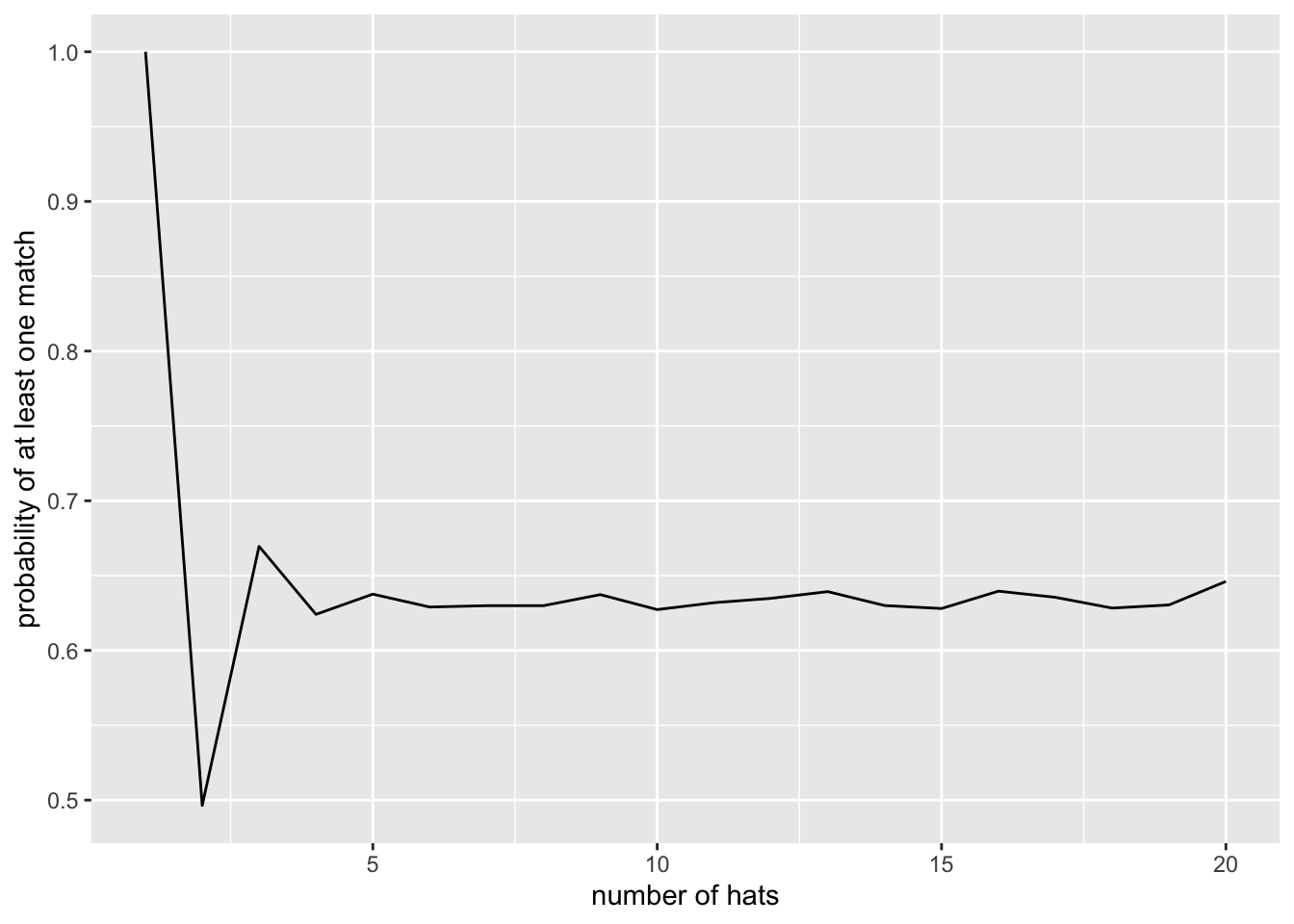

Example 3: Birthday Problem

What is the probability that in a room of 28 people, at least 2 of them have the same birthday?

Step 1: representing the birthdays

set.seed(7474)
class_birthdays <- sample(c(1:365), size = 28, replace = TRUE)
class_birthdays

 [1]  65 340 246 244 355 248 298 271 363 173 307 260 195 300 189 154 319  51 139
[20] 241 275 271 102 363 201 165  35  13

Step 2: any duplicates?

duplicated(class_birthdays)

 [1] FALSE FALSE FALSE FALSE FALSE FALSE FALSE FALSE FALSE FALSE FALSE FALSE
[13] FALSE FALSE FALSE FALSE FALSE FALSE FALSE FALSE FALSE  TRUE FALSE  TRUE
[25] FALSE FALSE FALSE FALSE

sum(duplicated(class_birthdays))

[1] 2

Function

class_duplicates <- function(unicorn) {
  class_birthdays <- sample(c(1:365), size = 28, replace = TRUE)
  num_duplicates <- sum(duplicated(class_birthdays))
  return(if_else(num_duplicates > 0, 1, 0))
}

class_duplicates()

[1] 0

class_duplicates()

[1] 1

Iterate

map_dbl(c(1:10), class_duplicates)

 [1] 0 1 0 0 0 0 0 0 1 0

Improve

class_duplicates <- function(class_size) {
  class_birthdays <- sample(c(1:365), size = class_size, replace = TRUE)
  num_duplicates <- sum(duplicated(class_birthdays))
  return(if_else(num_duplicates > 0, 1, 0))
}

set.seed(47)
num_stud <- 28
map_dbl(c(1:10), \(w) class_duplicates(class_size = num_stud))

 [1] 0 1 0 1 1 1 1 0 1 0

Many classrooms

set.seed(47)
num_stud <- 28
num_class <- 1000
map_dbl(c(1:num_class), \(w) class_duplicates(class_size = num_stud)) |>
  mean()

[1] 0.649

Vary number of students

set.seed(47)
num_stud_upper <- 28
num_class <- 100

birth_match_prob <- function(num_stud, reps) {
  prob <- map_dbl(c(1:reps), \(w) class_duplicates(class_size = num_stud)) |>
    mean()
  return(data.frame(match_prob = prob, num_stud = num_stud))
}

map(c(1:num_stud_upper), birth_match_prob, reps = num_class) |>
  list_rbind()

   match_prob num_stud
1        0.00        1
2        0.00        2
3        0.00        3
4        0.00        4
5        0.03        5
6        0.03        6
7        0.04        7
8        0.06        8
9        0.11        9
10       0.13       10
11       0.14       11
12       0.18       12
13       0.18       13
14       0.25       14
15       0.25       15
16       0.32       16
17       0.37       17
18       0.43       18
19       0.44       19
20       0.40       20
21       0.43       21
22       0.47       22
23       0.48       23
24       0.47       24
25       0.61       25
26       0.67       26
27       0.63       27
28       0.66       28

Visualize

set.seed(123)
num_stud_upper <- 40
num_class <- 1000

map(c(1:num_stud_upper), birth_match_prob, reps = num_class) |>
  list_rbind() |>
  ggplot(aes(x = num_stud, y = match_prob)) +
  geom_line() +
  labs(y = "probability of birthday match", x = "number of students in class")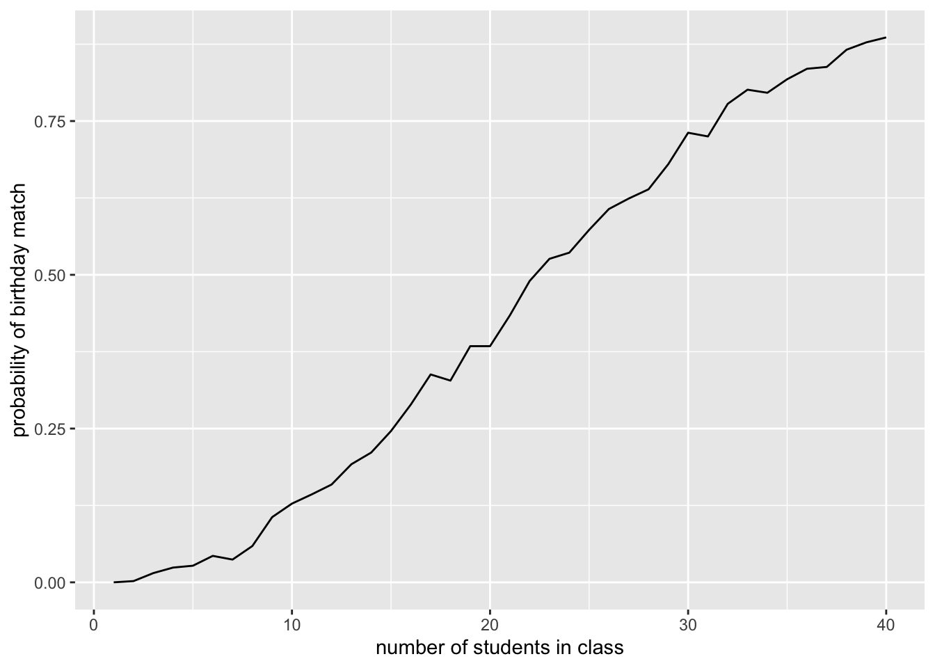

Good simulation practice

avoid magic numbers
set a seed for reproducibility
use meaningful names
add comments

Agenda 10/22/25

Simulating for model sensitivity

Simulate to…

… estimate probabilities (easier than calculus).
… understand complicated models.

Goals of Simulating Complicated Models

The goal of simulating a complicated model is not only to create a program which will provide the desired results. We also hope to be able to write code such that:

The problem is broken down into small pieces.
The problem has checks in it to see what works (run the lines inside the functions!).
uses simple code (as often as possible).

Bias in a model

Population:

talent ~ Normal (100, 15)
grades ~ Normal (talent, 15)
SAT ~ Normal (talent, 15)

The example is taken directly (and mostly verbatim) from a blog by Aaron Roth Algorithmic Unfairness Without Any Bias Baked In.

Goal for admitting students

College wants to admit students with

talent > 115

… but they only have access to grades and SAT which are noisy estimates of talent.

Plan for accepting students

Run a regression on a training dataset (talent is known for existing students)
Find a model which predicts talent based on grades and SAT
Choose students for whom predicted talent is above 115

Flaw in the plan …

there are two populations of students, the Reds and Blues.
Reds are the majority population (99%), and Blues are a small minority population (1%)
the Reds and the Blues are no different when it comes to talent: they both have the same talent distribution, as described above.
there is no bias baked into the grading or the exams: both the Reds and the Blues also have exactly the same grade and exam score distributions

What is really different?

But there is one difference: the Blues have more money than the Reds, so they each take the SAT twice, and report only the highest of the two scores to the college. This results in a small but noticeable bump in their average SAT scores, compared to the Reds.

Key aspect:

The value of SAT means something different for the Reds versus the Blues

(They have different feature distributions.)

Let’s see what happens …

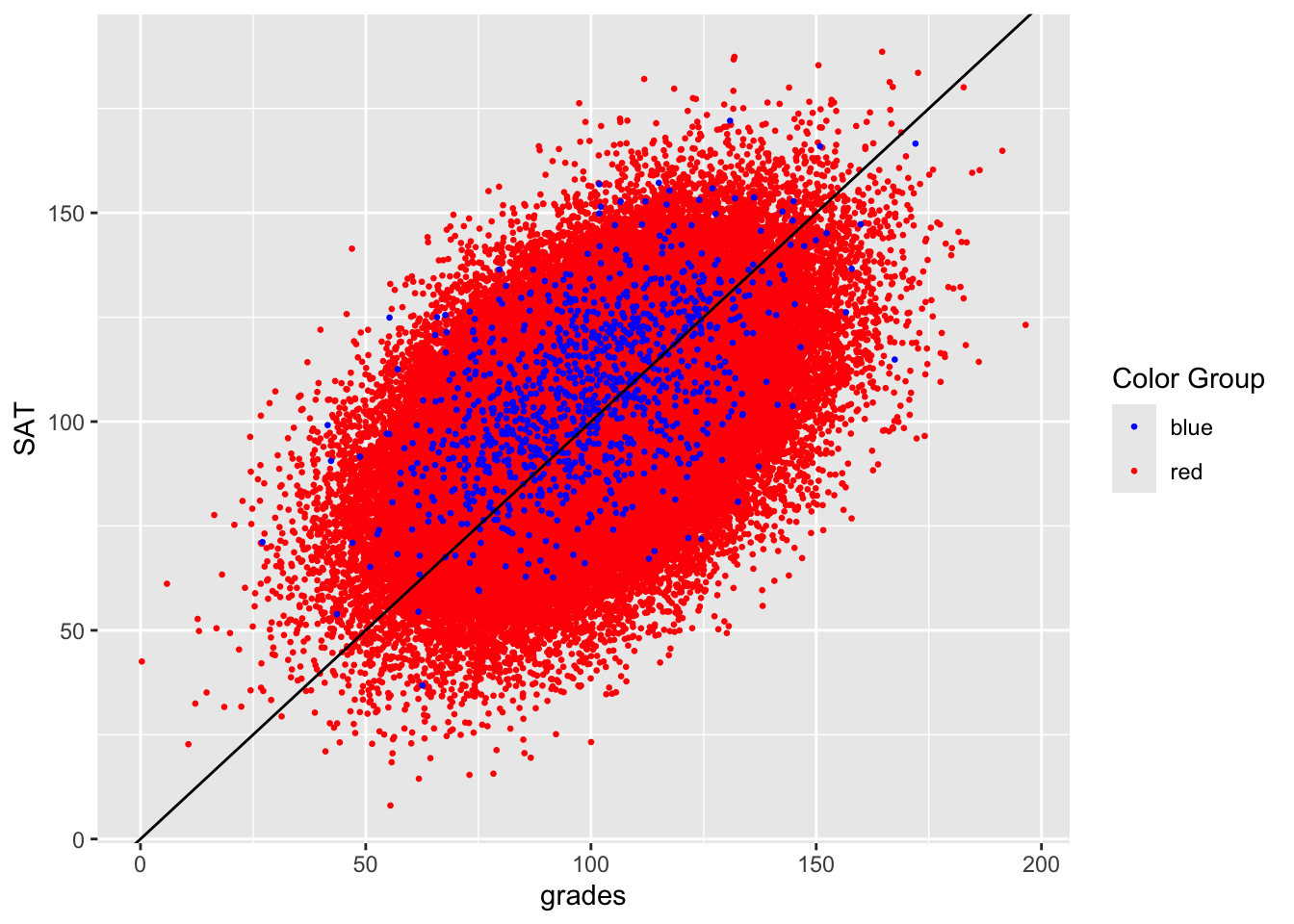
Two models:

Red model (SAT taken once):

# A tibble: 3 × 5
  term        estimate std.error statistic p.value
  <chr>          <dbl>     <dbl>     <dbl>   <dbl>
1 (Intercept)   33.2     0.152        218.       0
2 SAT            0.334   0.00149      224.       0
3 grades         0.334   0.00149      225.       0

Blue model (SAT is max score of two):

# A tibble: 3 × 5
  term        estimate std.error statistic   p.value
  <chr>          <dbl>     <dbl>     <dbl>     <dbl>
1 (Intercept)   25.3      1.60        15.8 2.04e- 50
2 SAT            0.432    0.0161      26.7 3.35e-119
3 grades         0.277    0.0154      18.0 6.83e- 63

New data

Generate new data, use the two models separately.
Can the models predict if a student has talent > 115?

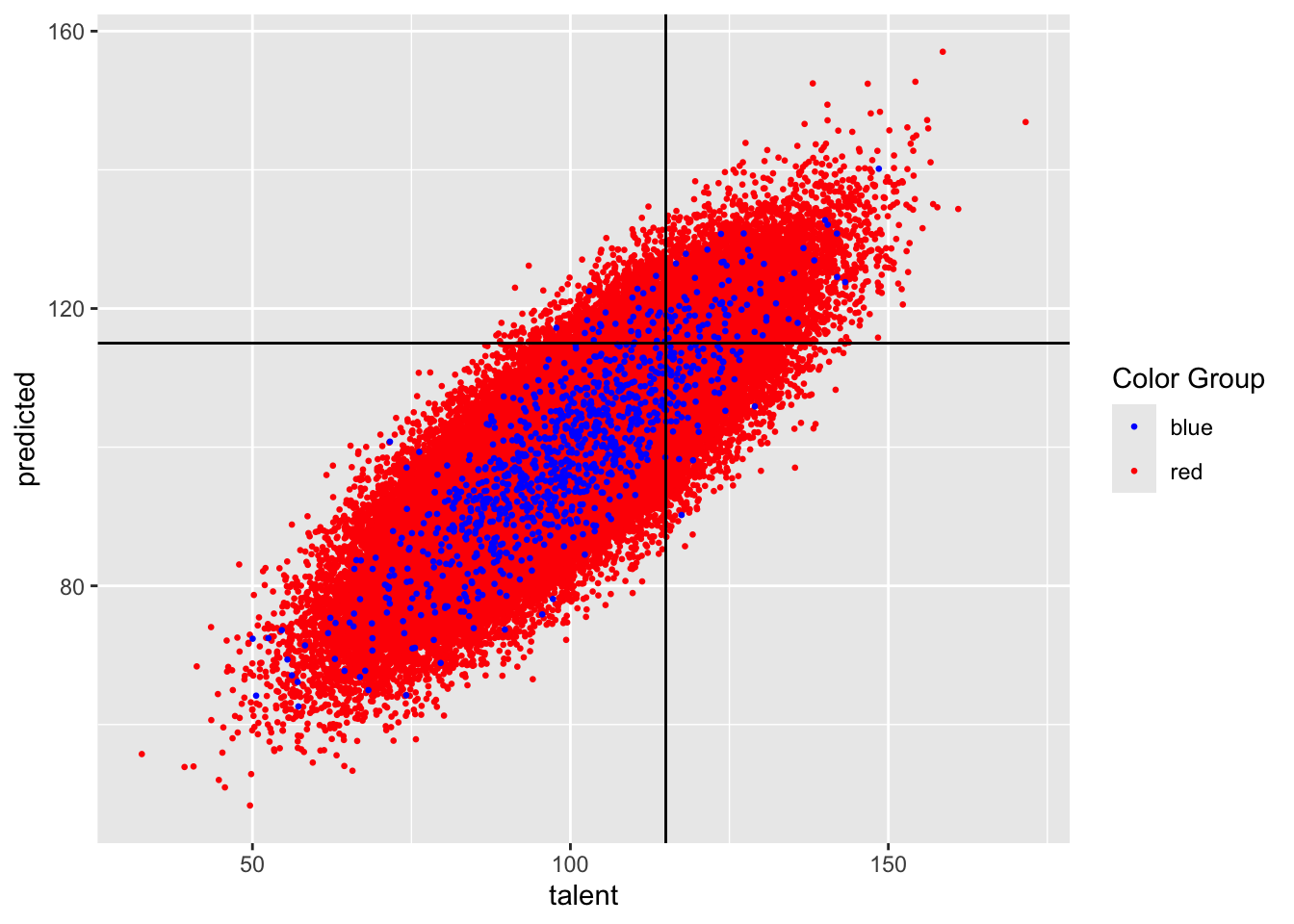
New data

# A tibble: 2 × 5
  color   tpr    fpr   fnr error
  <chr> <dbl>  <dbl> <dbl> <dbl>
1 blue  0.503 0.0379 0.497 0.109
2 red   0.509 0.0378 0.491 0.109

TWO models doesn’t seem right????

What if we fit only one model to the entire dataset?

After all, there are laws against using protected classes to make decisions (housing, jobs, money loans, college, etc.)

# A tibble: 3 × 5
  term        estimate std.error statistic p.value
  <chr>          <dbl>     <dbl>     <dbl>   <dbl>
1 (Intercept)   33.1     0.151        219.       0
2 SAT            0.334   0.00148      225.       0
3 grades         0.334   0.00148      226.       0

(The coefficients kinda look like the red model…)

How do the error rates change?

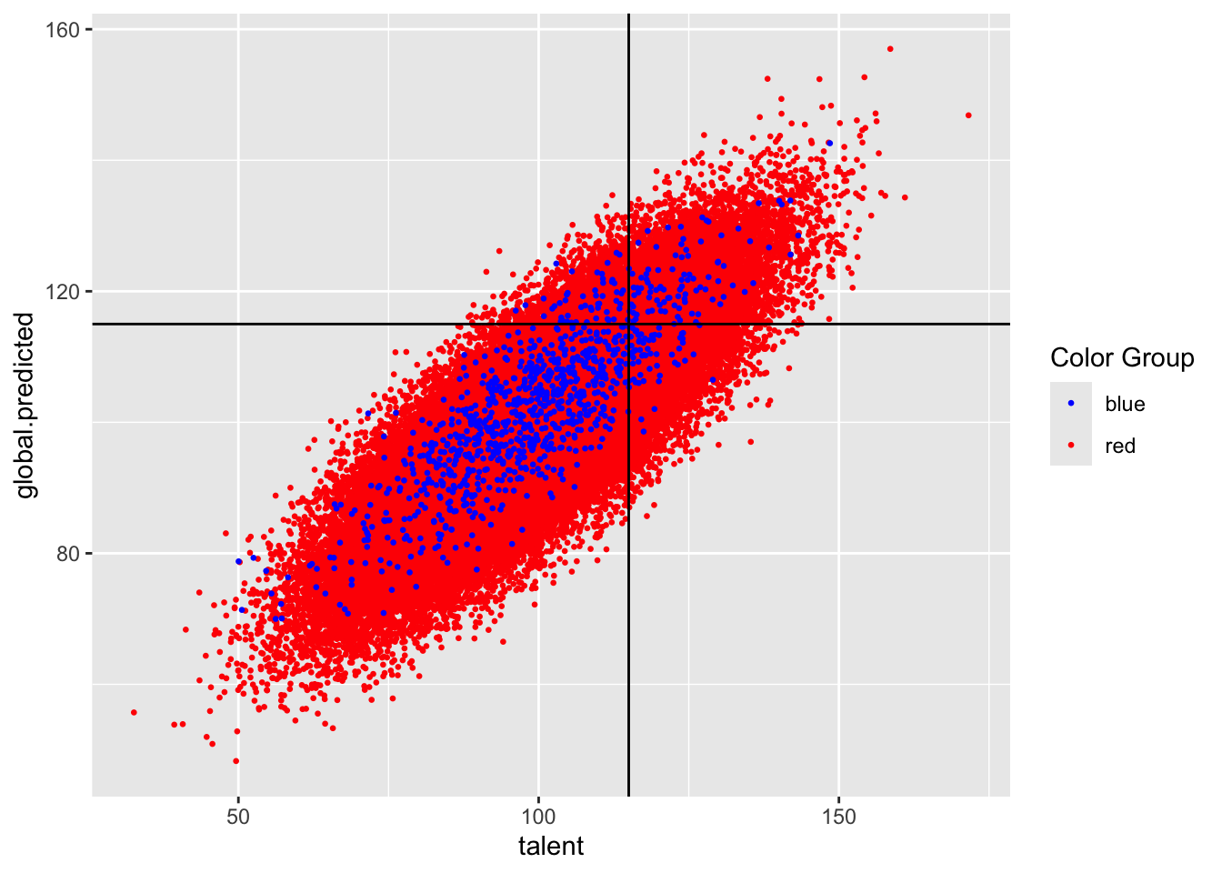
One model:

# A tibble: 2 × 5
  color   tpr    fpr   fnr error
  <chr> <dbl>  <dbl> <dbl> <dbl>
1 blue  0.619 0.0627 0.381 0.112
2 red   0.507 0.0375 0.493 0.109

Two separate models:

# A tibble: 2 × 5
  color   tpr    fpr   fnr error
  <chr> <dbl>  <dbl> <dbl> <dbl>
1 blue  0.503 0.0379 0.497 0.109
2 red   0.509 0.0378 0.491 0.109

What did we learn?

with two populations that have different feature distributions, learning a single classifier (that is prohibited from discriminating based on population) will fit the bigger of the two populations

depending on the nature of the distribution difference, it can be either to the benefit or the detriment of the minority population
no explicit human bias, either on the part of the algorithm designer or the data gathering process
the problem is exacerbated if we artificially force the algorithm to be group blind
well-intentioned “fairness” regulations prohibiting decision makers form taking sensitive attributes into account can actually make things less fair and less accurate at the same time

Simulate?

different varying proportions
effect due to variability
effect due to SAT coefficient
different number of times the blues get to take the test
etc.

Asset allocation

repeatedly run a model on a simulated outcome based on varying inputs
inputs are uncertain and variable.
output is a large set of results, creating a distribution of outcomes rather than a single point estimate.
easy to change the conditions of the models by varying the distribution type or properties of the inputs.

Taken from Risk Analysis Using Monte Carlo Simulations in R.

Aside: `rnorm()`

rnorm() calculates random normal values

rnorm(3)

[1] 1.0598770 0.2813142 0.1483487

rnorm(3, mean = 0, sd = 1)

[1] -1.5222088 -0.2609479  0.1393759

rnorm(4, mean = 47, sd = 5)

[1] 48.91283 45.11651 50.69179 42.14037

Asset allocation

Task: to model an asset allocation problem where you decide what portion of wealth should be allocated to risk-free investment or high-risk investment

the function calculates returns based on different asset allocations.

calculate_return <- function(step, alpha) {
  risk_free_rate <- 1.03
  risky_rate <- rnorm(1, mean = 0, sd = 1) * 0.05 + 1
  return(data.frame(
    step = step,
    return_rate = (1 - alpha) * risk_free_rate + alpha * risky_rate
  ))
}

calculate_return("unicorn", 0.47)

     step return_rate
1 unicorn    1.034815

Let alpha = 0.5

(half risky, half risk free)

decision_steps <- 12

pmap(
  data.frame(step = c(1:decision_steps), alpha = rep(0.5, decision_steps)),
  calculate_return
) |>
  list_rbind()

   step return_rate
1     1   1.0244265
2     2   0.9740712
3     3   1.0111959
4     4   1.0382488
5     5   1.0019058
6     6   0.9847674
7     7   1.0296142
8     8   0.9924038
9     9   1.0381949
10   10   1.0088956
11   11   1.0370043
12   12   1.0107057

Many runs

runs <- 10
decision_steps <- 12

run_func <- function(run, steps, alpha) {
  pmap(
    data.frame(step = c(1:steps), alpha = rep(alpha, steps)),
    calculate_return
  ) |>
    list_rbind() |>
    cbind(run_number = as.factor(run))
}

run_func("happy", 12, 0.5)

   step return_rate run_number
1     1   0.9972576      happy
2     2   1.0503818      happy
3     3   1.0133106      happy
4     4   1.0305766      happy
5     5   1.0424264      happy
6     6   1.0278066      happy
7     7   1.0088744      happy
8     8   1.0280513      happy
9     9   1.0270015      happy
10   10   1.0495620      happy
11   11   1.0483569      happy
12   12   1.0089000      happy

map(c(1:runs), run_func, steps = decision_steps, alpha = 0.5) |>
  list_rbind()

    step return_rate run_number
1      1   1.0037332          1
2      2   1.0305053          1
3      3   1.0177365          1
4      4   0.9851848          1
5      5   1.0200471          1
6      6   0.9777514          1
7      7   1.0139097          1
8      8   1.0394459          1
9      9   1.0311656          1
10    10   1.0111325          1
11    11   1.0600142          1
12    12   0.9529528          1
13     1   1.0511925          2
14     2   1.0188551          2
15     3   1.0546398          2
16     4   1.0286009          2
17     5   1.0090312          2
18     6   1.0116230          2
19     7   0.9982508          2
20     8   1.0397553          2
21     9   0.9748453          2
22    10   0.9994628          2
23    11   1.0325967          2
24    12   1.0265163          2
25     1   0.9846161          3
26     2   1.0106626          3
27     3   1.0085478          3
28     4   1.0253148          3
29     5   0.9879959          3
30     6   1.0761028          3
31     7   1.0095107          3
32     8   1.0417969          3
33     9   1.0299429          3
34    10   1.0483370          3
35    11   1.0039636          3
36    12   1.0177251          3
37     1   0.9957903          4
38     2   1.0446025          4
39     3   1.0151633          4
40     4   1.0208127          4
41     5   1.0138992          4
42     6   1.0241599          4
43     7   0.9636553          4
44     8   1.0330971          4
45     9   1.0707355          4
46    10   1.0341161          4
47    11   1.0076286          4
48    12   1.0437015          4
49     1   1.0166442          5
50     2   1.0424126          5
51     3   0.9944647          5
52     4   0.9669553          5
53     5   1.0152975          5
54     6   1.0145272          5
55     7   1.0372179          5
56     8   1.0407917          5
57     9   0.9811040          5
58    10   1.0213106          5
59    11   0.9962674          5
60    12   1.0518327          5
61     1   0.9804384          6
62     2   1.0313983          6
63     3   1.0456102          6
64     4   1.0019782          6
65     5   0.9848773          6
66     6   1.0166534          6
67     7   1.0338028          6
68     8   1.0222348          6
69     9   0.9802758          6
70    10   1.0156817          6
71    11   1.0424656          6
72    12   1.0575701          6
73     1   1.0750144          7
74     2   1.0058097          7
75     3   0.9927478          7
76     4   1.0009444          7
77     5   1.0055233          7
78     6   1.0573874          7
79     7   0.9575212          7
80     8   0.9957913          7
81     9   1.0893832          7
82    10   1.0135442          7
83    11   1.0152496          7
84    12   1.0331392          7
85     1   1.0304361          8
86     2   1.0111527          8
87     3   1.0077437          8
88     4   1.0031964          8
89     5   1.0507032          8
90     6   0.9713326          8
91     7   1.0101054          8
92     8   1.0556004          8
93     9   0.9991680          8
94    10   1.0232786          8
95    11   1.0182200          8
96    12   0.9987042          8
97     1   1.0250592          9
98     2   1.0300056          9
99     3   0.9890955          9
100    4   1.0395173          9
101    5   1.0147912          9
102    6   1.0243437          9
103    7   0.9964191          9
104    8   1.0782102          9
105    9   0.9746246          9
106   10   1.0194040          9
107   11   1.0383502          9
108   12   1.0508320          9
109    1   1.0563048         10
110    2   0.9850083         10
111    3   1.0395162         10
112    4   0.9711030         10
113    5   1.0193429         10
114    6   1.0259306         10
115    7   0.9889117         10
116    8   1.0418063         10
117    9   1.0055857         10
118   10   1.0155720         10
119   11   1.0350093         10
120   12   0.9916229         10

Cummulative product

numbers <- sample(1:5)
numbers

[1] 5 4 2 1 3

cumprod(numbers)

[1]   5  20  40  40 120

Cummulative rates

map(c(1:runs), run_func, steps = decision_steps, alpha = 0.5) |>
  list_rbind() |>
  group_by(run_number) |>
  mutate(compound_return = cumprod(return_rate))

# A tibble: 120 × 4
# Groups:   run_number [10]
    step return_rate run_number compound_return
   <int>       <dbl> <fct>                <dbl>
 1     1       0.984 1                    0.984
 2     2       1.01  1                    0.990
 3     3       1.04  1                    1.03 
 4     4       0.987 1                    1.02 
 5     5       1.04  1                    1.05 
 6     6       1.04  1                    1.09 
 7     7       0.994 1                    1.09 
 8     8       1.01  1                    1.10 
 9     9       1.01  1                    1.12 
10    10       0.994 1                    1.11 
# ℹ 110 more rows

Returns over time

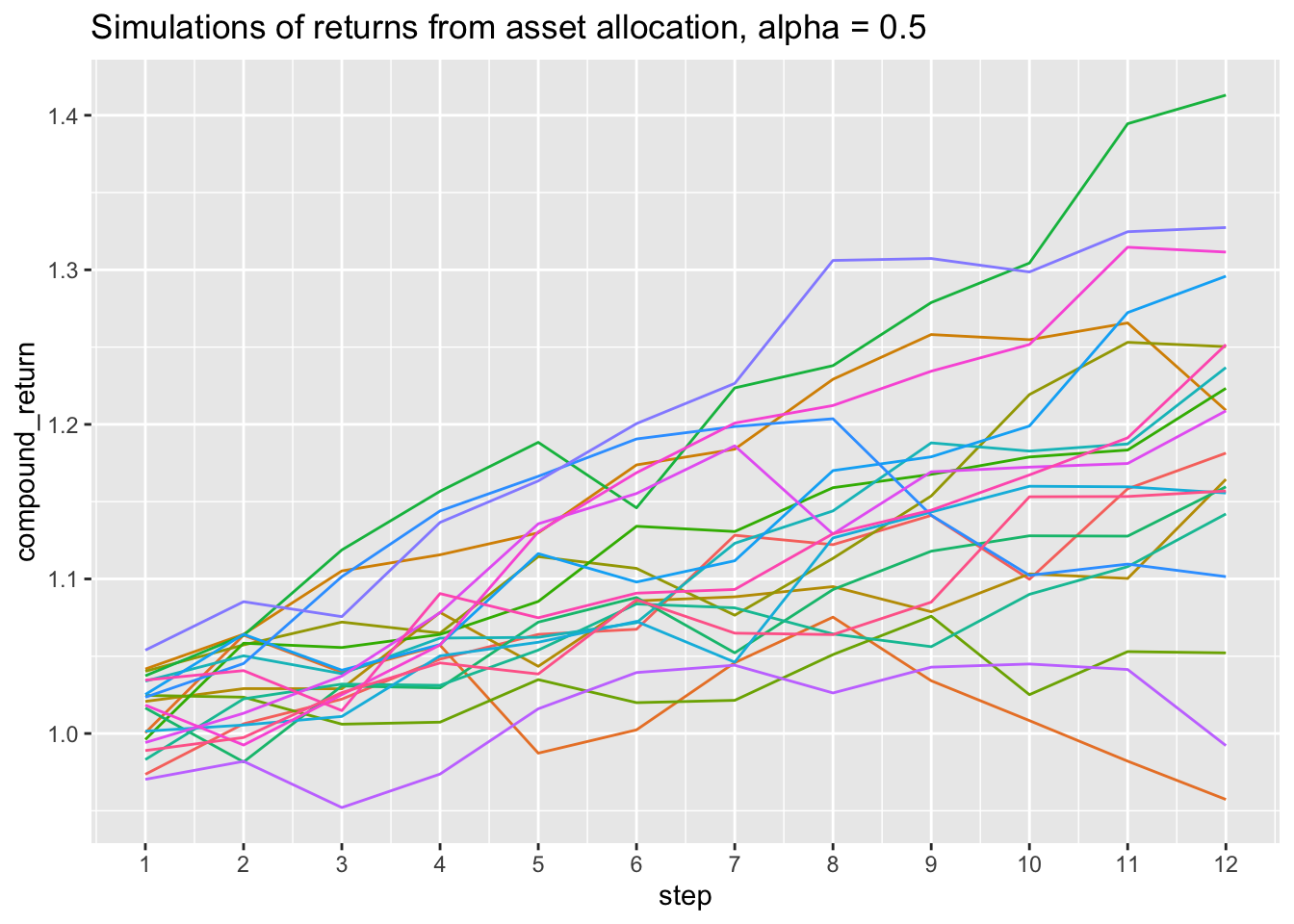
runs <- 20
map(c(1:runs), run_func, steps = decision_steps, alpha = 0.5) |>
  list_rbind() |>
  group_by(run_number) |>
  mutate(compound_return = cumprod(return_rate)) |>
  ggplot(aes(x = step, y = compound_return)) +
  geom_line(aes(color = run_number)) +
  theme(legend.position = "none") +
  scale_x_continuous(breaks = seq(1, 12)) +
  labs(title = "Simulations of returns from asset allocation, alpha = 0.5")

Change the allocation

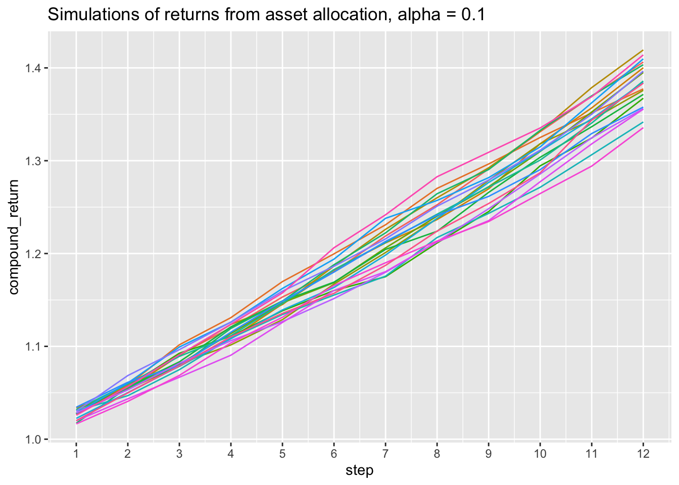
runs <- 20
map(c(1:runs), run_func, steps = decision_steps, alpha = 0.1) |>
  list_rbind() |>
  group_by(run_number) |>
  mutate(compound_return = cumprod(return_rate)) |>
  ggplot(aes(x = step, y = compound_return)) +
  geom_line(aes(color = run_number)) +
  theme(legend.position = "none") +
  scale_x_continuous(breaks = seq(1, 12)) +
  labs(title = "Simulations of returns from asset allocation, alpha = 0.1")

Change the allocation

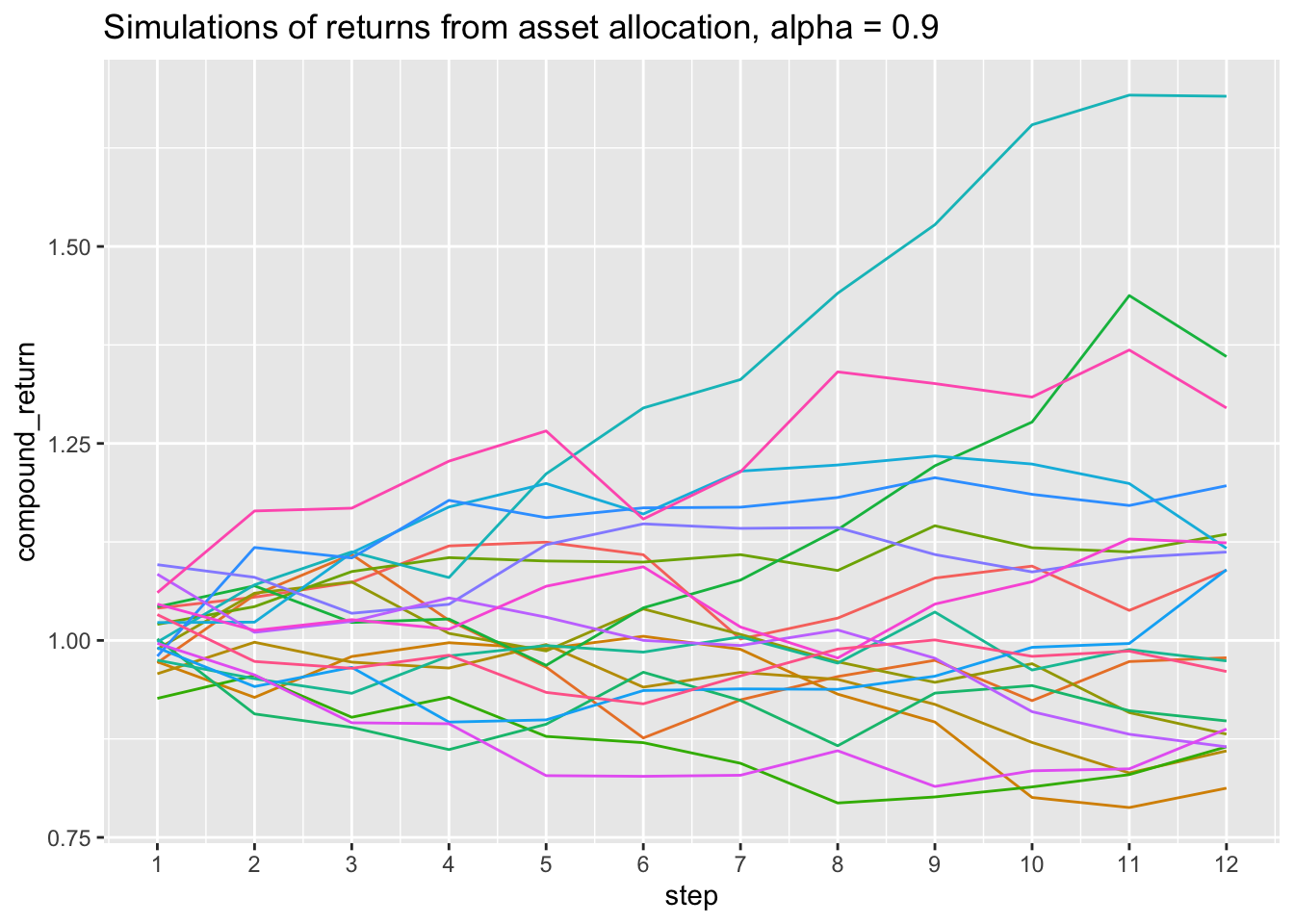
runs <- 20
map(c(1:runs), run_func, steps = decision_steps, alpha = 0.9) |>
  list_rbind() |>
  group_by(run_number) |>
  mutate(compound_return = cumprod(return_rate)) |>
  ggplot(aes(x = step, y = compound_return)) +
  geom_line(aes(color = run_number)) +
  theme(legend.position = "none") +
  scale_x_continuous(breaks = seq(1, 12)) +
  labs(title = "Simulations of returns from asset allocation, alpha = 0.9")

Change the return

calculate_return_sd10 <- function(step, alpha) {
  risk_free_rate <- 1.03
  risky_rate <- rnorm(1, mean = 0, sd = 10) * 0.05 + 1
  return(data.frame(
    step = step,
    return_rate = (1 - alpha) * risk_free_rate + alpha * risky_rate
  ))
}

calculate_return("unicorn", 0.47)

     step return_rate
1 unicorn    0.987021

run_func_sd10 <- function(run, steps, alpha) {
  pmap(
    data.frame(step = c(1:steps), alpha = rep(alpha, steps)),
    calculate_return_sd10
  ) |>
    list_rbind() |>
    cbind(run_number = as.factor(run))
}

Does the change impact long-term?

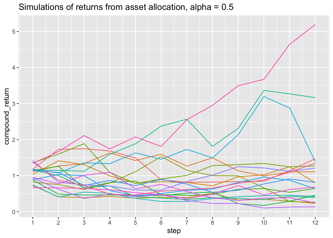
runs <- 20
map(c(1:runs), run_func_sd10, steps = decision_steps, alpha = 0.5) |>
  list_rbind() |>
  group_by(run_number) |>
  mutate(compound_return = cumprod(return_rate)) |>
  ggplot(aes(x = step, y = compound_return)) +
  geom_line(aes(color = run_number)) +
  theme(legend.position = "none") +
  scale_x_continuous(breaks = seq(1, 12)) +
  labs(title = "Simulations of returns from asset allocation, alpha = 0.5")

References

Baumer, Ben, Daniel Kaplan, and Nicholas Horton. 2021. Modern Data Science with r. CRC Press. https://mdsr-book.github.io/mdsr2e/.

Mosteller, Frederick. 1987. Fifty Challenging Problems in Probability with Solutions. Dover Publications: Mineola, NY.

Reuse

CC-BY-SA-4.0

Other Formats

Agenda 10/20/25

Data Conclusions

Simulate to…

Aside: if_else()

Aside: case_when()

Aside: sample()

Aside: set.seed()

Example 1: Alex & Jordan

Simulate their meeting

Results

Visualizing the meet up

Example 2: hats

Step 1: representing the hats

Step 2: everyone draws a hat

Step 3: who got their original hat?

Code so far

Function

Iterate

Reproducible

Vary number of hats

Vary number of hats

Visualizing

Example 3: Birthday Problem

Step 1: representing the birthdays

Step 2: any duplicates?

Function

Iterate

Improve

Many classrooms

Vary number of students

Visualize

Good simulation practice

Agenda 10/22/25

Simulate to…

Goals of Simulating Complicated Models

Bias in a model

Goal for admitting students

Plan for accepting students

Flaw in the plan …

What is really different?

Key aspect:

Let’s see what happens …

Two models:

New data

New data

TWO models doesn’t seem right????

How do the error rates change?

What did we learn?

Simulate?

Asset allocation

Aside: rnorm()

Asset allocation

Let alpha = 0.5

Many runs

Cummulative product

Cummulative rates

Returns over time

Change the allocation

Change the allocation

Change the return

Does the change impact long-term?

References

Reuse

Aside: `if_else()`

Aside: `case_when()`

Aside: `sample()`

Aside: `set.seed()`

Aside: `rnorm()`